Introduction

import libcarna
import matplotlib.pyplot as plt

Meshes

Using polygonal geometries is useful, for example, to create markers or to generally enrich visualizations. In 3D graphics, meshes are used to define polygonal geometries. We start with the definition of a mesh for a cube:

cube = libcarna.meshes.create_box(40, 40, 40)

The size of the cube is given in scene units (SU), and here it is 40 SU in width, height, and depth. Scene units can be anything that we agree them to be, like micrometers (e.g., for visualization of cellular image data) or millimeters (e.g., for image data from computer tomography). It is only important that they are used consistently.

Next, we define some materials:

green = libcarna.material('solid', color=libcarna.color.GREEN)
red   = libcarna.material('solid', color=libcarna.color.RED  )

Materials determine how meshes (i.e. polygonal gemetries) are rendered. In LibCarna, a material consists of a shader and a set of parameters like colors. Supported shaders comprise solid for materials whose colors are affected by light (the default), and unshaded for materials that are colored uniformly.

Scenes

Now that we have a mesh and some materials in place, we can create a scene that defines some spatial relations. We create two spatial geometry objects, both using the cube mesh, but with different colors:

GEOMETRY_TYPE_OPAQUE = 1

root = libcarna.node()

libcarna.geometry(
    GEOMETRY_TYPE_OPAQUE,
    parent=root,
    mesh=cube,
    material=green,
).translate(-10, -10, -40)

libcarna.geometry(
    GEOMETRY_TYPE_OPAQUE,
    parent=root,
    mesh=cube,
    material=red,
).translate(+10, +10, +40)

<libcarna._spatial.geometry.<locals>.Geometry at 0x7c02b5141eb0>

Scenes are defined hierarchically, so they form a tree-like structure. The local coordinate system of a node always is defined with respect to the coordinate system of its parent node. In this example, the green cube is moved by -10 SU along the x- and y-axes, and by -40 SU along the z-axis. The red cube is moved in the opposite direction.

Note on GEOMETRY_TYPE_OPAQUE: A geometry type is an arbitrary integer constant, that establishes a relation between the geometry nodes of a scene, and the corresponding rendering stages (see below).

Finally, we define a camera that will serve as the point of view for scene rendering:

camera = (
    libcarna.camera(parent=root)
    .frustum(fov=90, z_near=1, z_far=1000)
    .translate(z=250)
)

The frustum method defines the projection from 3D to planar coordinates. The fov argument defines the field of view of the camera in degrees. The z_near and z_far arguments define the distance of the near and far clipping planes to the camera; geometries, that are closer than 1 SU or farther than 1000 SU, will not be rendered.

Rendering

Now we are all set to perform the rendering — almost! One ingredient is missing: The renderer. We only have opaque geometries involved, so we set up the rendering pipeline accordingly:

opaque = libcarna.opaque_renderer(GEOMETRY_TYPE_OPAQUE)
r = libcarna.renderer(500, 370, [opaque])

Each renderer can have an arbitrary number of rendering stages. Here, we only use the opaque rendering stage to render all geometries in the scene that we have annotated with the GEOMETRY_TYPE_OPAQUE as the geometry type.

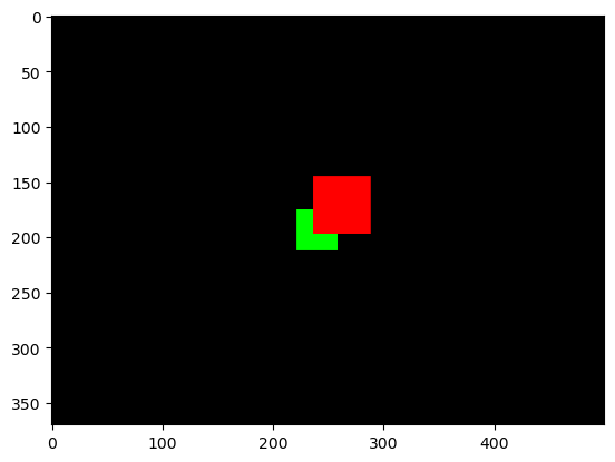
And then it’s time to render. We can inspect the result with matplotlib, for example:

img = r.render(camera)
plt.imshow(img)

<matplotlib.image.AxesImage at 0x7c02b4fff890>

Animations

It is much easier to visually grasp the information in a 3D scene by looking at it from different angles. For this reason, there is a set of convenience functions that fascilitates creating animations, by rendering multiple frames at once:

# Define animation
animation = libcarna.animate(
    libcarna.animate.rotate_local(camera),
    n_frames=50,
)

# Render and show animation
libcarna.imshow(animation.render(r, camera))

In this example, the camera is rotated around the center of the scene (more precisely: around it’s parent node, that happens to be the root node of the scene). The scene is rendered from 50 different angles. For each angle, the result is a NumPy array.

Use libcarna.imshow to view animations, matplotlib does not work nicely.